

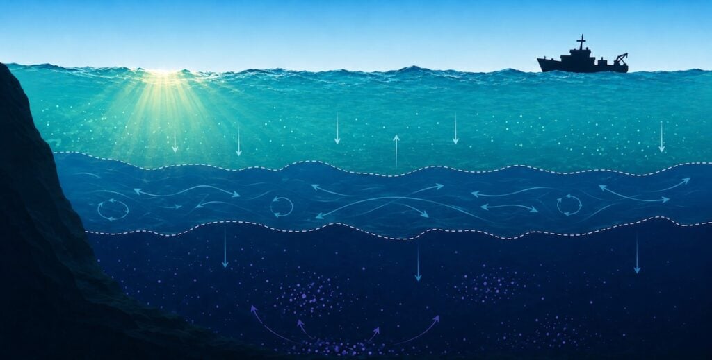
Sound velocity conditions can change while a hydrographic survey is still underway, meaning a profile that accurately represented the water column when collected may become outdated as conditions evolve. Read more >>
In an ongoing series of discussions with Jonathan Beaudoin of HydroOctave Consulting, AML Oceanographic examines why profiling frequency needs to reflect environmental variability rather than rely solely on predetermined time intervals, and how hydrographers can recognize conditions that may call for additional sampling.
Beaudoin’s work in multibeam sonar informs much of the discussion, including the distinction between precision and accuracy, the limitations of fixed profiling intervals, and the role of real-time observations in determining when another sound velocity profile may be needed.
How Sound Velocity Affects Survey Accuracy
Underwater sound does not travel along a straight path. Sound waves refract as they pass through layers with different temperature and salinity characteristics, creating two potential sources of error. Refraction can distort the estimated position at which a sonar beam reaches the seafloor, while scaling can distort the calculated distance traveled along the ray path.
In multibeam survey data, these effects can appear as “smiles” or “frowns,” with the edges of the swath curving upward or downward. Such patterns indicate that the seafloor may not be mapped accurately and can result in rework and safety risk.
When the sound velocity (SV) profile is outdated, too sparse, or miscalibrated, both depth and position can be compromised. The resulting bias is systematic and repeatable, and post-processing cannot fully correct a dataset affected by inaccurate sound velocity information.
This makes profiling frequency an important part of managing survey accuracy. Data can appear clean while retaining an underlying bias if changing oceanographic conditions have not been sampled frequently enough.
Precision Does Not Necessarily Mean Accuracy
A hydrographic dataset can be internally consistent and smooth while still carrying residual bias if sound velocity conditions have not been fully captured.
Following correction, gridded bathymetry may show reduced distortion and acceptable statistical metrics. However, smiles and frowns are visible symptoms of undersampling. Processing away those symptoms does not correct the underlying gap in sound velocity coverage, meaning the resulting data may appear improved without fully representing the true seafloor.
Precision in this context describes how well the data agrees with itself. A single survey pass can therefore be precise because there is no independent pass against which it has yet been compared.
Repeatability can only be tested with a second, independent pass over the same area. That second pass may also be internally precise while failing to align with the first. Assuming all other sources of error and bias are well managed, accurate sound velocity information is necessary for the two passes to agree.
The objective is therefore accuracy rather than precision alone, with profiling frequency playing an important role in achieving it. Beaudoin explores these principles further through his Multibeam Crash Course.
Matching Profiling Frequency to Ocean Variability
There is no single profiling interval appropriate for every survey. Although one cast every two hours is a commonly used default, conditions may require more frequent sampling.
The relevant factor is how quickly the oceanographic environment is changing. If sound velocity varies faster than profiles are collected, bias can accumulate and persist for extended periods before it is detected.
Traditional casting methods create an operational tradeoff. Collecting additional profiles can improve the representation of changing conditions, but each cast can introduce downtime and associated operational costs. If neither downtime nor budget increases were involved, surveyors could profile much more frequently. In practice, every cast competes with productivity.
A practical approach is therefore to identify a “Goldilocks” frequency. Too few profiles increase the risk of systematic bias, while profiling too often can reduce operational efficiency. The appropriate interval sits between these extremes and should reflect observed environmental variability rather than an arbitrary period of time.
A hybrid approach can establish a fixed baseline while increasing sampling frequency as oceanographic conditions change. This remains a guide rather than a guarantee and, with traditional methods, still assumes that additional casts require additional time and expenditure.
Underway profiling systems change this tradeoff by reducing the downtime associated with collecting profiles. Tools such as the Moving Vessel Profiler (MVP) can therefore reduce operational costs while allowing continuous underway sampling, improving accuracy without sacrificing efficiency.
Moving Beyond Minimum Sampling Requirements
Client specifications may establish minimum SV sampling intervals, but those intervals are not necessarily sufficient to achieve the accuracy required under the conditions encountered during a particular survey.
An end client might, for example, specify a minimum of four casts per day. Hydrographers should not necessarily treat that minimum as adequate under all conditions. Because they can observe conditions directly in the field, meeting a specified minimum does not remove the responsibility to collect additional profiles when necessary to achieve the required accuracy.
This places an emphasis on understanding the oceanographic environment rather than treating a contractual minimum as an automatically sufficient sampling strategy. Hydrographers can combine their knowledge of oceanography with observations made during acquisition when deciding whether profiling frequency needs to increase.
Oceanographic models may assist in anticipating variability, but acquisition also provides an opportunity to monitor conditions directly. Keeping survey systems active and examining incoming data can allow surveyors to identify patterns early, often through visual clues alone.
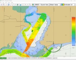
An example of a real-time map of surface sound speed, as read by the sound velocity sensor at the transducer. This map was created using QPS Qinsy 9.8.0. Maps like this provide a clear view of spatial patterns and help identify areas that may require closer attention.
Small inconsistencies, changes in surface sound speed behavior, or other features that do not appear as expected can provide early indications of sound velocity issues. Real-time maps of surface sound speed, using readings from the sound velocity sensor at the transducer, can also provide a clear view of spatial patterns and help identify areas that may require closer attention.
Recognizing Changes During the Survey Day
Local solar noon provides a practical example of why a fixed profiling interval may not adequately represent changing conditions.
During periods of peak solar heating, near-surface sound velocity can change more rapidly. Profiles can consequently age faster than at other times of day, and the sampling rate may need to be increased.
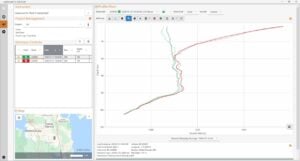
An illustrative example from Sailfish compares two casts collected at the same site 12 hours apart. Below approximately 40 m, the profiles correspond closely. Near the surface, however, they diverge in a manner consistent with solar heating over the course of the day.
The comparison illustrates how a morning cast may not reflect afternoon conditions near the surface, even when deeper water has not changed. Responding to this type of variability, rather than relying on the clock alone, is central to determining an appropriate profiling frequency.
Quantifying Changes Between Profiles
Environmental variability can also be assessed quantitatively. An approach developed by Beaudoin alongside NOAA and Woolpert involves calculating the harmonic sound speed for each cast and comparing it with the preceding profile.
A large difference between casts can indicate that more frequent profiling is needed.
NOAA’s experimental Moby Sound Speed TPU Estimator applies this concept in the field. Survey teams using the approach have adjusted their casting intervals accordingly, including one case in which the interval was relaxed from every two hours to every four hours.
The example demonstrates how profiling intervals can be adjusted in response to measured conditions rather than relying exclusively on a predetermined schedule.
Profiling According to Operational Risk
The available margin for error also influences how closely environmental variability needs to be tracked.
Higher-risk operations involving safety of navigation provide less tolerance for falling behind changing oceanographic conditions than a lower-stakes task such as a quick localization job.
Different survey applications may therefore justify different profiling frequencies.
The appropriate profiling frequency can consequently depend on the application, observed environmental variability, incoming survey data, and the consequences of residual error.
Sound velocity errors can often be identified during acquisition through artifacts or inconsistencies in survey data. The challenge is interpreting and resolving those signals correctly. When profiling is too infrequent, or environmental changes are not fully captured, residual bias can remain even after the most obvious visible issues have been addressed.
Managing sound velocity error therefore depends on keeping sampling aligned with the rate at which the ocean is changing. Rather than treating a minimum number of casts or a fixed interval as inherently sufficient, profiling frequency provides hydrographers with a practical means of managing the risk that changing water-column conditions introduce into survey accuracy.